Root system architecture impacts row crop emissions
At Hi Fidelity Technologies, our root phenotyping device (called RootTracker) was used to interrogate many scientific questions, but there was one question that intrigued us most of all: do differences in root system architecture lead to differences in greenhouse gas emissions?
Why is this plausible in the first place? Let us consider maize. Maize requires a large nitrogen application, often ammonium nitrate. While it is possible to target the application of fertilizer to a specific location, usually it is just sprayed onto the soil surface. Some of that nitrogen will be absorbed by the plant, but a large portion of it will not. Ultimately, the unabsorbed fertilizer runs into water or decomposes, giving off nitrous oxide (N2O) in the process.
Nitrous oxide is a major greenhouse gas. It is the third largest contributor after carbon dioxide (CO2) and methane, and is nearly 300 times more potent than CO2 (IPCC and Wuebbles). Row crop agriculture is by far the largest source of anthropogenic N2O emissions (Reay et al. and the EPA).
If one could identify cultivars with root system architecture that did a better job acquiring fertilizer, then one could reduce N2O emissions. The plants would be better and so would the environment.
And it is not only maize that is a major N2O emitter. Soybean production results in N2O emissions as well. Together, soybean and corn make up an enormous amount of US agriculture — over 75% of acres planted (USDA). Clearly, finding cultivars with lower emissions profiles could reduce N2O emissions in a major way.
Experiment
The experiment took place in the summer of 2021 and 2022 near Ames, IA. I will only go into the results for 2021, since that year of work was completely public- and self-funded and made use of proprietary germplasm, but the results for 2022 aligned with the 2021 results.
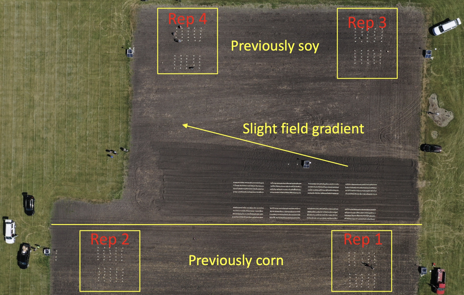
We grew maize at one location using two proprietary hybrids (i.e. two types of maize seed) — HFG1071 and HFG1111. There were four blocks, one plot per variety within each block. These four blocks tried to capture variance across both previous crop as well as soil type. Each plot had 5 rows. 25 equally spaced RootTracker devices were placed on plants within the plot. I will use the terms rep and block interchangeably here.
In the present post, I won’t go into the details of how RootTracker measures root growth, which can be found here. The key thing is that RootTracker measures the amount of root growth over time in terms of the number of root touches per day (within a certain depth band).
Measuring N2O is tricky. Traditionally and the way we did it in this experiment, one puts a “collar” in each plot, which is just a wide, short tube like a bit of 12” PVC. To measure the N2O emissions, one attaches a lid to the tube for a while, and then pulls out some gas, which is sent to the lab for an assay. (In our 2022 experiment, we were actually able to use a laser to take instantaneous in-field measurements.) Part of the challenge is that N2O emissions are known to be sporadic with certain events like rainfall leading to large belches of N2O. Further, emissions outside of the growing season may matter as well. In 2021, we were able to take roughly weekly measurements in June and July.
Results
As mentioned previously, N2O emissions can be event driven. For instance, rainfall leads to big belches of N2O. Conversely, when it is dry for extended periods, there is likely very little emissions. We saw this in 2021, when July was a very dry month and we recorded minimal emissions. For that reason, I will focus on June when there was enough rainfall to produce non-trivial emissions data.
Below you will find the June, 2021 emissions vs. root growth. The “rate” of root growth is the number of detections divided by amount of device uptime within a period of interest (in days). We normalize by time because the devices can have slightly different uptimes — e.g. a battery might need to be replaced, so a device does not collect data for several hours. For each rep and variety, I have computed a trimmed mean (10% symmetric trim) of rates over all devices in a plot.
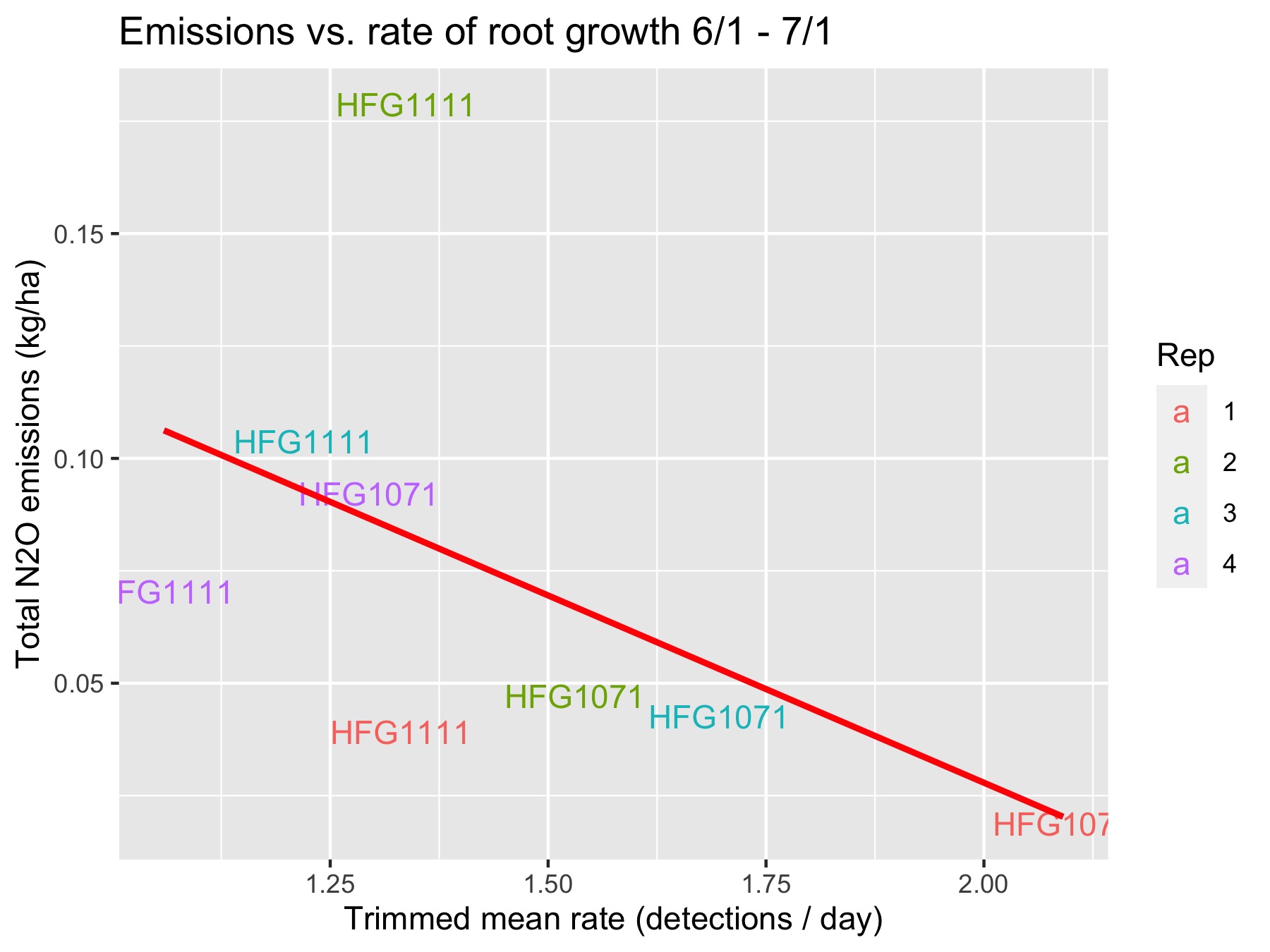
Two things immediately jump out:
- On an absolute basis, there is an inverse relationship between the amount of emissions and amount of roots. In other words, more roots correlates with less emissions, regardless of variety or block.
- For 3/4 of the blocks, HFG1071 has more root growth and less emissions, so we also see this pattern on a relative basis. And for the one block in which this does not occur, both hybrids have relatively low root growth.
We can quantify these differences. Regarding the first point, after running a linear regression we find that for every additional root grown per day the monthly emissions are reduced by -0.083 kg/ha (p=0.18). If we remove the outlying point, then this becomes -0.067 kg/ha (p=0.049) — a lower effect size, but with less uncertainty.
Regarding the second point, we want to understand if varietal differences in root growth could be used to drive differences in emissions. Running a mixed model where variety is a fixed effect and the rep is a random effect, we find that HFG1111 has 25% less root growth compared to HFG1071 (-0.41 roots/day less compared to 1.68 roots/day for HFG1071, p=1e-5). In other words, the two hybrid varieties do seem to have noticeably different patterns of root growth in this experiment.
Keep in mind that this is one month in one location in one year. We should be careful to draw conclusions from such a limited experiment. As with yield, interactions with the environment can have a big impact on results, and we have seen cultivar by environment interactions in other experiments. But the early evidence does lend itself to the idea that root system architecture impacts emissions and that this might be exploited to chose cultivars with lower greenhouse gas costs. (Sadly, we had to shut our doors before we could adequately test this hypothesis.)
Conclusion
This is just one example of an analysis I would conduct at Hi Fidelity Technologies. We ran many experiments both for ourselves and for clients. Other questions we addressed include:
- How do root systems respond to drought, and how does that vary with genetics?
- Do biostimulant seed treatments impact root growth, and is there an interaction with the environment?
- How does herbicide tolerance manifest itself in root growth?
Each experiment we ran demanded its own unique analysis, but there are certain tools that are frequently used. The linear model and variants are ubiquitous: mixed models if there are random effects, quantile regression if there are outliers or potentially an unusual distribution of error terms, or spatial models when trying to capture variations due to soil or other slowly varying environmental factors.
While I am not a partisan for any particular statistical philosophy, one of the nice things about the Bayesian perspective is that it easily encompasses all of these methods in one framework. And one of the major advantages of working with a linear model is that it provides interpretable results. The most important thing at the end of the day is being able to capture a result in a narrative that is easy to understand.