Inferring root growth using RootTracker

At the startup I used to worked for, Hi Fidelity Genetics, I helped invent a patented technology to measure root growth using impedance sensing called RootTracker. If we conceptualize a root as a random walk, it was like our device could observe one point along this trajectory. Given only that information, we wanted to describe differences in root structure between varieties and recapitulate root growth over time.

This post is based on the paper, “Inferring monocotyledon crown root trajectories from limited data.”

Background

RootTracker

Below is a picture of our circular RootTracker. It has a cylindrical symmetry. The green, vertical “paddles” are printed circuit board. Each paddle has 22 gold plated electrodes that act as sensors running down the side. You place a seed in the center of a device and let it grow. We measure voltages at the sensors and convert them to detections using an algorithm. We describe this and early data in more detail in our paper “Capturing in-field root system dynamics with RootTracker”.

Using RootTracker detection data, we could quantify differences between varieties and over time. However, this does not provide an actual representation of root growth using a model. While there are several quite complex models out there to simulate root growth, like OpenSimRoot, they are not applicable for our data, which is rather limited. These simulation-based models seek to recapitulate root growth in the most realistic way possible. Parameters of those models can be tweaked to learn how they impact hypothetical root growth, but they cannot be easily used to make inferences. In contrast, our attempt at modeling started with the goal of making inferences and from there we tried to build a model that could recapitulate root growth.

Monocot root growth

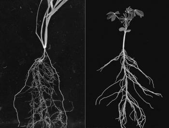
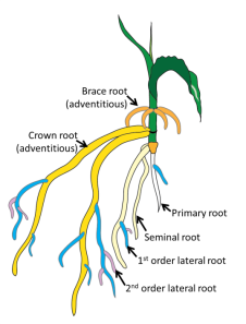
In the picture above we have drawn a corn plant inside of the device. The system works with both monocots (like corn, wheat, and rice) and dicots (like soybean and cotton). For the purposes of modeling though, we will restrict our attention to monocots. In the black and white image below, we see a monocot (young wheat) on the left and a dicot (young lupin) on the right. Dicots have a tap root off of which roots grow. In contrast, monocots have crown roots that emerge at the stem of the plant near the soil-surface interface effectively giving us an origin for root emergence, which is useful for modeling. In the color image, we see a cartoon of monocot root growth. RootTracker can detect both crown roots and lateral roots. For the sake of simplicity, we just assume that all roots detected are crown roots. The images below are reproduced from Plants in Action, published by the Australian Society of Plant Scientists.

Methods

Data we use here came from an experiment at Alamance Community College in Alamance, NC in early 2022. The aim of the experiment was to compare root growth of maize, wheat, soybean, cotton, and tomato. Here we will just focus on maize and wheat. (We use the terms maize and corn interchangeably.) Five gallon pots were filled with soil. A RootTracker device was placed into the soil and then a seed was placed in the soil at the center of the RootTracker. Each treatment had 24 RootTrackers.

Data Exploration

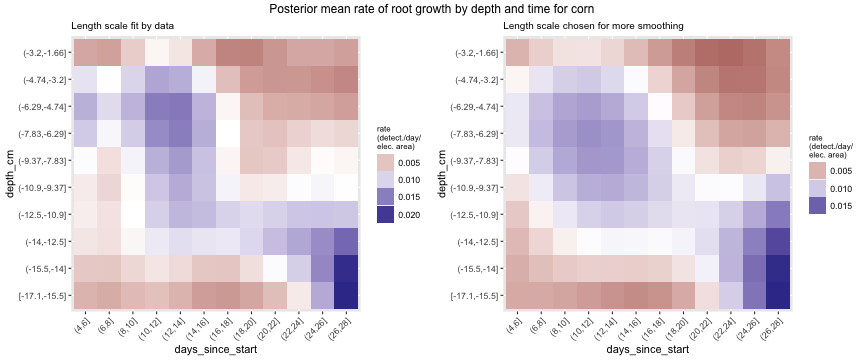
Using just our detection data and no modeling, we can examine how root growth changes over time. Below we plot maize root growth over time, after having been smoothed using a Gaussian process. The image on the left is fit using cross validation, while the image on the right uses hyperparameters that impose more smoothing. In both images there seems to be more root growth at the middle depths early on and then root growth concentrates at greater depths as time goes on. Further, we see two majors times of root growth, first around days 10-14 and later around days 24-28. Having a periodic pattern to root growth makes sense for monocots, since the several crown roots emerge simultaneously in what are called whorls.

Model

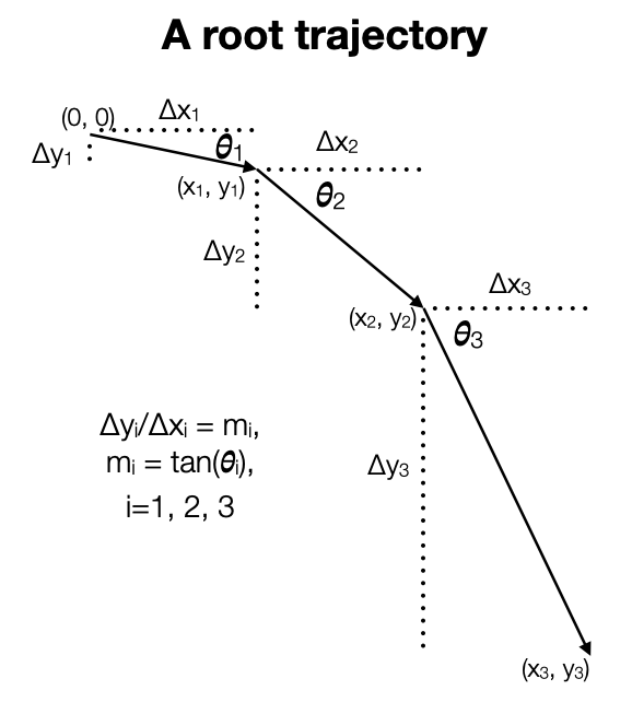
Our model is motivated by gravitropism. A root grows in a given direction for a period and then changes direction, presumably a direction that is a little steeper than before. Below we have a picture of that process. We considered two different approaches to modeling. First, we considered modeling changes in the slope, \(m_i, i = 1, 2, 3\). If the changes in slope are generally downward, then we get a root that moves generally downward. Second, we considered modeling changes in the angle \(\theta_i, i = 1, 2, 3\). If the changes in angle are generally downward, then we get a root that moves generally downward. (The choice of three pieces here is arbitrary.)

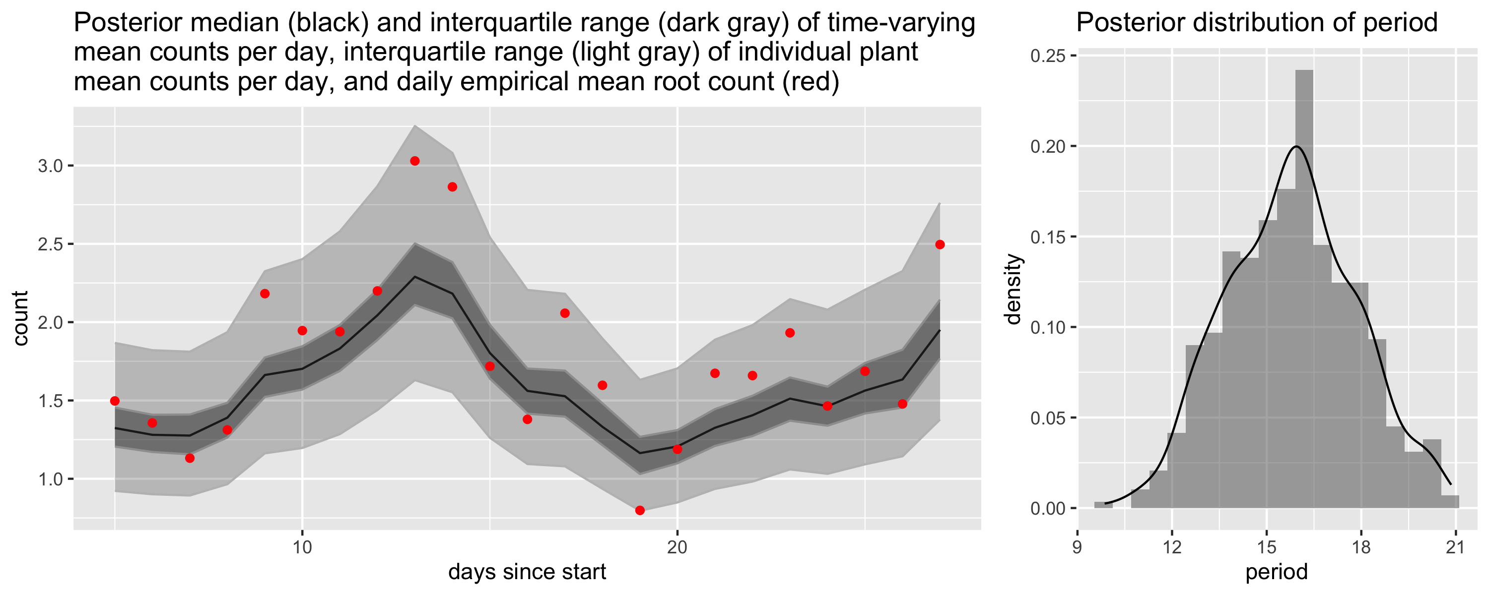
We modeled the time of emergence separately from the depth. In particular, we modeled the counts using a binomial model where the time-varying probability of root emergence was modeled on the log-odds scale using a Gaussian process with a periodic kernel. In the plot we show the expected number of roots to emerge each day. You can see that we capture the two periods of heightened root growth between days 10-14 and 24-28. The plot on the right shows the posterior for the period parameter, which is roughly two weeks.

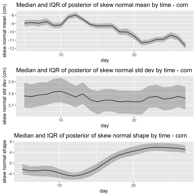
We also introduce time varying parameters when modeling the depth distribution. We tried several alternatives for modeling the changing slopes or angles. Below we show the results when modeling the changing slopes using a skew normal distribution. You can see that both the mean and shape of these distributions changes over time as the root growth goes from shallower to deeper.

Recapitulating root growth

We can bring all of this statistical modeling together to recapitulate root growth. Below, we show a video of “canonical” root systems from this experiment for corn (top) and wheat (bottom).