Using AI to extract root detections
Introduction
At Hi Fidelity Technologies, we were interested in measuring root growth. Roots are critical for nutrient and water uptake, but they have long been ignored because roots are difficult to measure. We invented and developed a novel device called RootTracker, which could measure root growth using something akin to capacitance touch sensing. That may sound easy, but it was a slog. The basic problem is that roots are made up of mostly water, and they are in a medium that is mostly water (and opaque). How do you detect water in water?
Here I am going to walk you through two different answers to that question. The first is a physics answer, while the second is a data science answer. I’ll spend most of my time on the data science answer, since that is where I did the most work, but I’ve got to give a shout out to my colleage, Jeff Aguilar and his physics based approach, since it is what originally cracked the problem.
Background
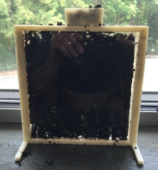
Below is a picture of a RootTracker device. There is a circuit encased in urethane at the top, which houses the microprocessors that drive the device. Emanating out of the urethane are printed circuit board “paddles”, which have 22 gold plated electrodes running down the edge. An individual electrode is charged up and then voltage at that elected is measured. This is done for all 22 electrodes on all 12 paddles for 2 different charging times every 5 minutes, resulting in something like a 2x12x22 dimensional time series of voltages. We want to figure out how to use those voltages to identify when a root passes near a sensor.
![]()
Using physics to identify roots
This problem was first dealt with by Jeff Aguilar, Hi Fidelity’s lead engineering. Jeff has a physics background and it was incredibly informative to see a talented physicist like Jeff think. Jeff would tackle a problem using a mix of both theory and experimentation. Theory, in the sense of trying to define models or metrics that capture the dynamics of whatever is being observed. Experimentation, in the sense of trying to identify and bifurcate the factors that might be driving the system. He was also a master of visualization, making plots or movies to gain intuition. Let us start with the experimentation and then go to the theory.
Experimentation
One of our biggest challenges was identifying ground truth. How do you identify when a root passes by a sensor if you cannot see it? Jeff came up with an ingenious solution to that problem, dubbed an “ant farm experiment.”
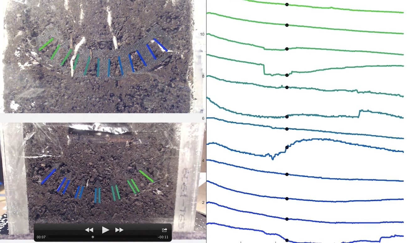
Below is a picture of an “ant farm.” It consisted of a 3d-printed frame, which sandwiched soil between two pieces of plexiglass. A corn seed was placed in the tiny box on top. When it germinated its early roots would grow through the ant farm.
Embedded in the soil were electrodes, which were attached to a microcontroller to record their voltages. The electrodes can be seen here as the blue-to-green lines in the left hand side of the image. On the right you can see the voltages over time, color coded to match up with their corresponding electrodes. Jeff placed a camera on either side of the ant farm and then synced the subsequent video with that of the time series so that you could monitor the point on the time series that corresponded to the current frame of the video. In that way, one could watch a root grow past a sensor and then see what it did in the time series. Using this methodology convinced us that when a root growing past a sensor could cause a disturbance in observed voltages.
Theory
The time series were largely smooth, but they displayed a variety of behavior. In addition to changes when a root grew past, the humidity of the soil could impact the signal, along with shifts in the soil, which were not uncommon. What, specifically, indicated the presense of a root? To answer that Jeff, developed a model circuit whose parameters included the local resistance and capacitance at a sensor. One could transform the voltage data to these resistance and capacitance parameters, so that one in effect was monitoring local resistance and capacitance at each sensor over time. Constructing videos in R-C space and then flagging times that corresponded to root activity found in the aforementioned videos, Jeff was able to identify “signatures” for when a root grew past a sensor. I am being very succinct in my description here, but that is the basic idea.
This was all a tremendous achievement, but it begs the question: how can we use AI/ML/statistics to pick the optimal “signature” of a root passing a sensor. That’s what we want to describe next.
Using data science to identify roots
Our aim at Hi Fidelity Genetics was to measure root growth in real world experiments, either in the greenhouse or in the field. Like before, we run into the same problem: how does one identify ground truth when one cannot see when a root passes a sensor? Here we will adopt a different approach than the “ant farm” experiment. Instead, we will conduct an experiment in which some devices have plants in them and some do not.
Let’s think about this for a second, because it is not obvious that it will work. We are collecting a 2x12x22 dimensional time series. Let’s say there are 8000 time points. In that case, we effectively have 2x12x22x8000 covariates for a binary (yes plant/no plant) response. We can observe tens to hundreds of plants. Thus, we have relatively few cases against a large number of covariates. Thankfully, using intuition guided by our knowledge of the physics approach, we can find a way to do this. And, we can also recover individual root touches in the process, which is to say the phenotype of interest, not just the binary response!
Data set
The data that we will be using throughout is from a greenhouse experiment that took place over the course of 1 month. We tested devices (like the one pictured in the Background section) with maize, wheat, soybean, cotton, and tomato plants in them as well as devices with no plants. There were 24 devices per treatment, including for the no plant control. For our purposes here, we will only focus on maize vs no plant.
Soil was placed in pots. RootTracker devices were inserted into the soil and a seed was placed at the center of the device, except for those devices with no plant. All pots were hand watered as necessary.
Data exploration
One of the first things that jumps out when looking at raw voltage data is that the two measurements are often highly correlated. Below, we randomly pick three electrodes from a device and plot the voltages for the two different charge times against one another. (The charge times are 1 and 255 microseconds respectively.)
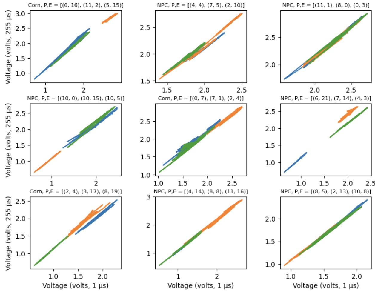
In effect, the voltages seem to be moving along a common manifold (a line in this case). At first glance, it seems like we might only need to use one of the voltages — why use both when they are highly correlated? But what we know from the physics approach is that key information comes from when there is movement off of the common manifold, which is to say when the voltages are diverging in some way. We want to get at that information. While the lines seem to have a very similar slope and position, they are not identical. Thus, we will treat each individually.
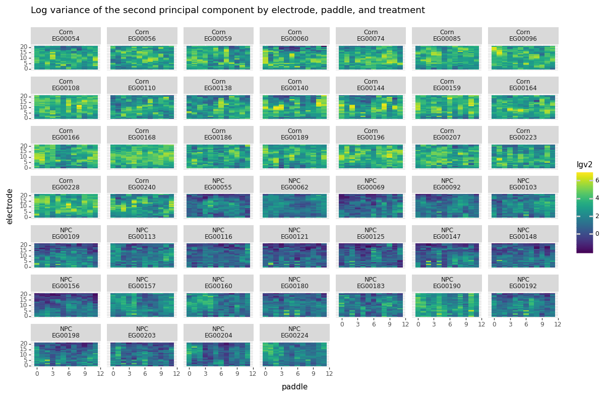
For each paddle and electrode, we compute the principal components decomposition of the time series of the two voltage measurements. Most of the variation will be in the first component, which captures the joint movement of the two time series. The second component captures how much the two time series are converging or diverging. A key element here is we want to orient the principal components decomposition so that the second component always corresponds to movement down and to the right and the first component always corresponds to movement up and to the right.
Below we plot the (log) variance found in the second principal component for each paddle and electrode. Keep in mind this is a global statistic constructed using all of the time points available. We see clear separation between the two groups, which is a good sign that monitoring the second component will indeed tell us something about when a root is passing by an electrode.
Let us conceptualize of the 2D time series as the trajectory of a particle over time. What we have done so far is for each paddle and electrode chosen a convenient and informative set of coordinates for tracking the trajectory. Now, we want to summarize the particle’s movement through time. To that end we will compute some statistics on a rolling basis. In particular, for each coordinate we will keep track of the mean and standard deviation of the instantaneous velocity over a set window, like 2 hours time. (We also measure the angular velocity) in 2D.
Below we plot the time series of these and other statistics: the mean location of coord. 1, the mean location of coord. 2, the mean veloicty of coord. 1, the mean velocity of coord. 2, the standard deviation of the velocity of coord. 1, the standard deviation of the velocity of coord. 2, the mean angular velocity, and the standard deviation in the angular velocity. I may call a velocity “momentum”, since the ideas are interchangeable.
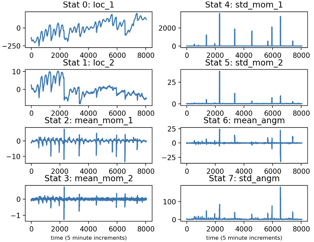
For each of these statistics, I found the 1st and 99th percentile globally, then I computed the time each device was either “low” or “high” on that basis for each statistic. Averaging over each group (corn / no plant), one finds that the extreme negative values for the mean velocity of the second component and the extreme high values for the standard deviation of the velocity of the second component are the most informative statistics.
All of this lead to the following algorithm:
- Identify periods of “anomalous” behavior, which is to say when there is large negative velocity in the second principal component. (We also enforce that the standard deviation must be above zero, but not too high, which corresponds to when we have a steady negative velocity.)
- Combine periods of time that are very close to one other in time or are on adjascent electrodes at similar times on the same paddle.
- Remove periods that occur simultaneously across paddles, which might correspond to when the plants are watered or some other global phenomenon. Also remove periods that are too short.
- Either integrate the total anomalous time or count the number of anomalous periods.
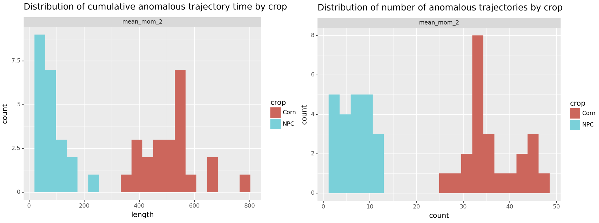
Doing that separates the two groups! Below we plot both metrics, either total anomalous time or number of anomalous periods. By either approach we see corn separate from the no plant control (NPC).
At this point, this is all a bit ad hoc. For instance, what are the optimal cutoffs for flagging a detection? We want to do some actual statistics to show that we can optimize this process, which is what we tackle next.
Using AI to flag roots
The first element of the algorithm above is to identify periods when the velocity of the second component are excessively low. Mathematically speaking, this is pretty straightforward, it is
\[f(x) = \begin{cases} 1, \; \text{ if } x < \tau \\ 0, \; \text{ else }. \end{cases}\]We can approximate this function via a sigmoid. In particular, if we let \(\sigma(x) = 1 / (1 + e^{-x})\), and \(g(x; \kappa) = \sigma(- \kappa (x - \tau))\) then
\[g(x; \kappa) \rightarrow f(x) \text{ as } \kappa \rightarrow \infty.\]In other words \(g\) is a soft threshold approximation of \(f\). In the language of neural networks, this is a linear layer followed by a sigmoid activation function. Thus, it should perhaps not be surprising that we can use this model to separate the two groups.
To be completely clear, we use a slightly more complicated model, but doing that, we can replicate the work above. In the language of PyTorch, our model (M1) is the following
nn.Sequential(
    SoftThreshold(),
    RemoveSimultaneous(),
    Integrate(sum_dim = (1, 2, 3)),
    nn.Linear(1,1),
    nn.Flatten(start_dim=0)
)
where SoftThreshold is akin to \(g\) above, RemoveSimultaneous tries to
remove periods high activation across multiple paddes (effectively (3) from
above), and Integrate (approximately) integrates the time above the threshold.
A slight modification (M2) of this is:
nn.Sequential(
    SoftThreshold(),
    RemoveSimultaneous(),
    Integrate(sum_dim = (1, 2, 3)),
    nn.Flatten(start_dim=1),
    nn.BatchNorm1d(1, momentum = 0.0),
    nn.Flatten(start_dim=0)
)
The BatchNorm1d layer is equivalent to the linear layer, but resolves a
technical issue that occurs when using the linear layer. Our batch consists of
the whole data.
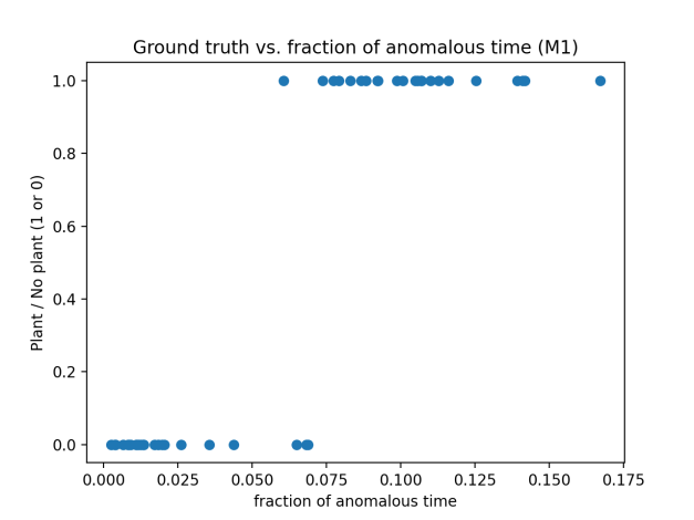
Instantiating the model M1 using values similar to those used in (1) above, we see that we can nearly separate the two groups.
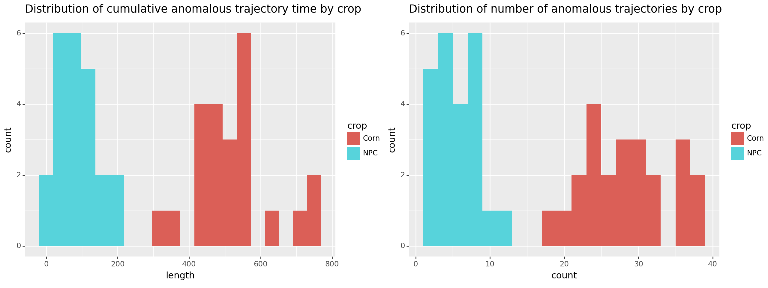
If we extract the activations from the very first layer, which is effectively the indicator being above the threshold, and filter as in steps (2), (3), and (4) we can completely separate the two groups and produce a picture very similar to the one above.
Lastly, using (M2), we can actually learn the parameters of interest. Below is the ground truth vs. log-odds plot after having optimized the parameters.
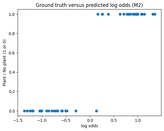
We have almost separated the two groups without even doing steps (2), (3), and (4). Comparing the cutoff value for the mean velocity using our ad hoc method compared to what we can learn via optimization, we find that the optimal parameter is slightly lower.
| ad hoc threshold | learned threshold |
|---|---|
| -0.25 | -0.29 |
Interestingly, though the ad hoc approach uses log variance between -2. and -1., after optimizing it lands between -3.27 and -2.93, considerably lower and quite a narrow range (0.20 to 0.23 in terms of standard deviation).
(Note, we have not used cross-validation here because we are fitting a 5 parameter model using 46 cases.)
Conclusion
It took some work, but we have shown that it is possible to create a model that learns its parameters solely from a binary response (yes plant / no plant) to recover root detection information. This proof-of-concept shows that one can extend this approch to construct larger models, e.g. deep neural networks, to learn more complex patterns that indicate the presense of a root or not.
If you are curious, the analysis above employes the following notebooks and a custom Python package (which is not yet published):