Gaussian conditioned on a piecewise affine, continuous function

Here is a problem that arose while we were modeling root growth in monocots (e.g. maize).

Suppose that a priori \(X \sim N(\mu, I_n)\). Subsequently, we learn that \(\ell(X) = 0\) where \(\ell\) is a piecewise affine, continuous function. How does one sample \((X \vert \ell(X) = 0)\)?

It turns out that you can sample this conditional distribution using Hamiltonian Monte Carlo (HMC). I have written up the methods in a paper, if you want to check out the details, and put together a Python package called ctgauss that does the sampling.

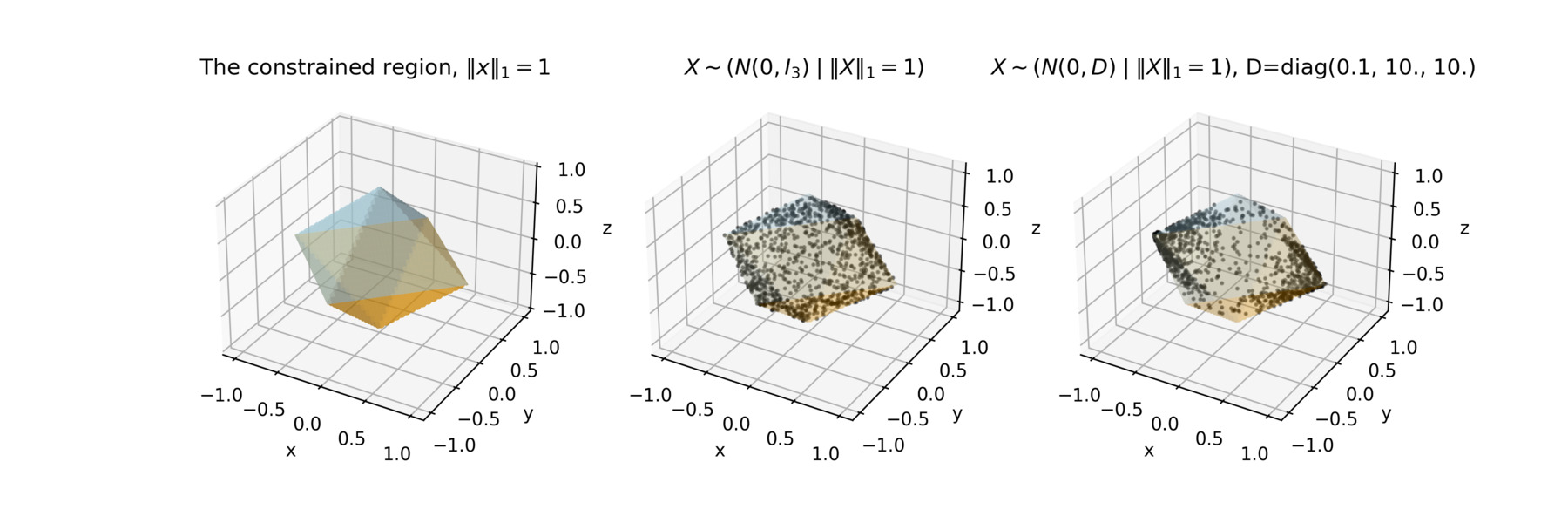
This lets you do things like sample \(X \sim (N(0, \Sigma) \; \vert \; \|X\|_1 = 1)\). In the figure below you will find this example for two different covariance structures. You can even use a piecewise quadratic log density, if you want.

Approach

In the paper, you will find that I have synthesized the work of Pakman and Paninski, who deal with truncations, and Mohasel Afshar and Domke, who deal with steps, and then place that within the context of a particle moving on a manifold within a higher dimensional space.

The key to all of this is that we know the exact dynamics of a particle when the log-density of the distribution of interest is piecewise quadratic. A piece on which our function is defined is determined by a finite number of hyperplanes. Since the dynamics are known exactly on that piece, we can compute the hypothetical time to reaching each boundary, the smallest time being the one that matters, since that is the one the particle will hit.

It is then just a matter of understanding the physics. If the particle encounters a hard wall or a change in potential that is greater then its kinetic energy, it will be reflected. Otherwise, it will “climb” over the potential, but lose some momentum in the process.

When to use ctgauss

If you hear “HMC”, you should immediately think Stan, which is an excellent piece of software for Bayesian inference using Hamiltonian Monte Carlo. In many modeling scenarios, Stan will work, even with truncations or for some non-smooth densities (see e.g. Stan’s function reference, section 3.7). For instance, you can sample approximately from the distribution above using the model below with data, e.g. list(N=3, y=1.), if you relax the requirement that the sample lie exactly on the surface \(\|X\|_1 =1\).

data {
	int<lower=1> N;
	real<lower=0> y;
}
parameters {
	vector[N] x;
}
transformed parameters {
	real z = sum(fabs(x));
}
model {
	for (i in 1:N) {
		x[i] ~ normal(0.0, 1.0);
	}
	y ~ normal(z, 0.01);
}

However, to the best of our knowledge and as of this writing, Stan may be unable to accommodate some use cases, like arbitrary truncations by hyperplane in multiple dimensions or when the piecewise affine, continuous function used for conditioning is complex, in which case ctgauss may be useful. (Or if you really, really want to sample on \(\ell\) and not near it.)

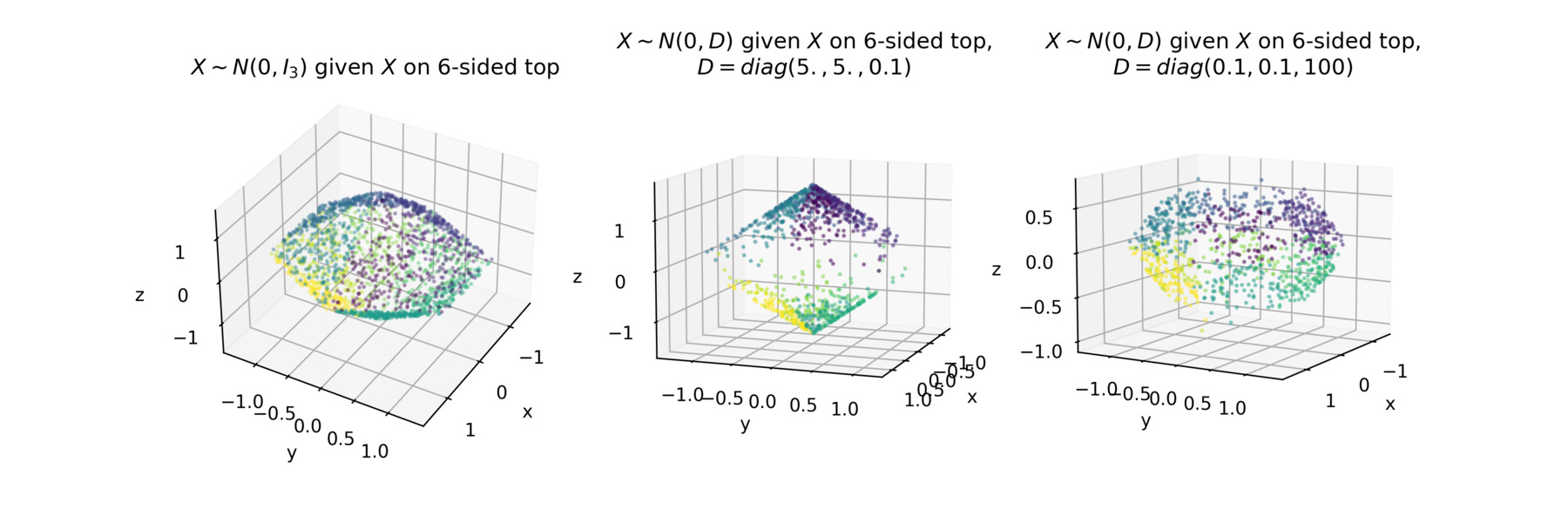
For instance, generalizing the example above, we can do the same thing for any n-sided top. Below we plot various samples on a 6-sided top using ctgauss.

Conclusion

The bottom line is, if you can use Stan, use it. If you have a weird use case, then consider ctgauss. Another upside to ctgauss is that it is easy to understand the code base. The paper includes an appendix with the algorithm, and that algorithm is closely mapped to what is actually implemented in Python, making it easy to hack the code, if you want.

Let me know if you have any questions!